Introduction

Our story starts from the paper “Tesco Grocery 1.0, a large-scale dataset of grocery purchases in London”. It presents a record of 420 millions food items purchased by 1.6 million fidelity card owners who shopped at the 411 Tesco stores in Greater London over the course of the entire year of 2015. The data is aggregated at multiple levels of census areas (borough, ward, MSOA, LSOA) to preserve anonymity.

In the paper, the authors describe the derivations of multiple food characteristics (associated to each area), mainly concerning the energy, weight, type and entropy of the bought products. The authors then establish the validity of the dataset by comparing food purchase volumes to population from official census and match nutrient and energy intake to official statistics of food-related illnesses. To find out more about the Tesco paper and its characteristics, do not hesitate to consult their official page.

Their dataset contains precious information concerning eating habits, indeed it is one of the only studies with such a big scale that contains both geo-location and nutritional information. This raised our interest and led us to wonder:

Have you ever heard sentences like “Healthy eating is a privilege of the rich”? Well, with the Tesco dataset we have the chance to bring further checking to this kind of claim and bring an element of answer to the more general question “Do wealthier populations buy healthier food?”

In order to answer our interrogation, we came up with the following questions:

• At MSOA level in Greater London, are there major differences in eating habits depending on the wealth level?
• Is there evidence of social class difference in eating habits?
• Do wealthier MSOA areas buy food that could be judged healthier?

As a side note and disclaimer, let us underline that the following analysis is done as part of the Applied Data Analysis course (EPFL) and that we wish to make this data story on a lighter tone than the core work. If you want to find all the serious explanations and details on the calculations, we advise you to read the corresponding notebook.

For our investigations, we will question DATA. It’s our best contact to get some insights on our questions.

Let’s present DATA

He knows everything about the Tesco Grocery dataset. DATA also has a friend that was issued by Greater London Authority. His friend contains a wide range of statistical information on MSOA’s population, including the median income that we want to use as a base for our wealth estimate. But DATA is quite voracious. After meeting his friend, he managed to merge him inside and find out the useful information contained in his friend that we needed.

DATA discarded information coming from MSOAs for which the ratio of people having a clubcard at Tesco among the total population of the area was not representative. DATA followed the same procedure as the original Tesco paper by discarding all MSOAs whose $representativeness_{normalized}$ was below $0.1$. This procedure leads to the removal of a little less than $10\%$ of the MOSAs.

A last fact we should know about DATA is that he perfectly knows the coordinates of every MSOA on the map below:

So now DATA will answer our questions but we need to ask the right ones! First, we would like to know more about the wealth classes.

DATA, what are the wealth classes?

DATA: “I used the median income by area as the main indicator of wealth. The median has the advantage of being robust to strong outliers (which is often the case with income because they usually follow a Pareto distribution). Then I ran PCA…”

That’s enough DATA, don’t bore us with the details and show us some stats!

DATA: “Ok ok, here are your stats…”

To recap:

• very low class areas have a median annual household income below 29’000£
• low class between 28’000£ and 36’000£
• medium class between 36’000£ and 45’000£
• high class between 45’000£ and 57’000£
• very high have a median income greater than 57’000 £

Finally, as we could expect, we see the number of areas with high and very high household income are much lower than the rest.

DATA, DATA, show me which population class eats healthy!

And let’s be clear DATA, from now on I don’t want you to talk, just show us nice and smooth answers to our questions!

Let’s consider for each MSOA, the set of nutrient weight as a vector. We will use T-SNE visualization to compare eating habits difference between each MSOA using these vectors. T-SNE model distances between vectors, so two MSOAs close to each other have similar vectors, whereas if they are far away to one another the vector are dissimilar. We will do the same with distribution of purchased product types.

DATA: “Please note that the colours correspond to wealth classes…”

DATA… do you remember what we just said?

Sadly, it seems they are no great clusters on these T-SNE visualisation… But it also seems DATA is trying to hide something from us. We can observe that there’s still a clear cluster for the very high class and that it does not overlap with the very low class in all visualizations.

Sorry DATA, but we will need to examinate you into more details…

Show us for example a map of London with both wealth classes and mean weight of consumed fibre in each MSOA. It is a fairly accepted fact that fibre is a good indicator of healthy diet so maybe we’ll get an insight.

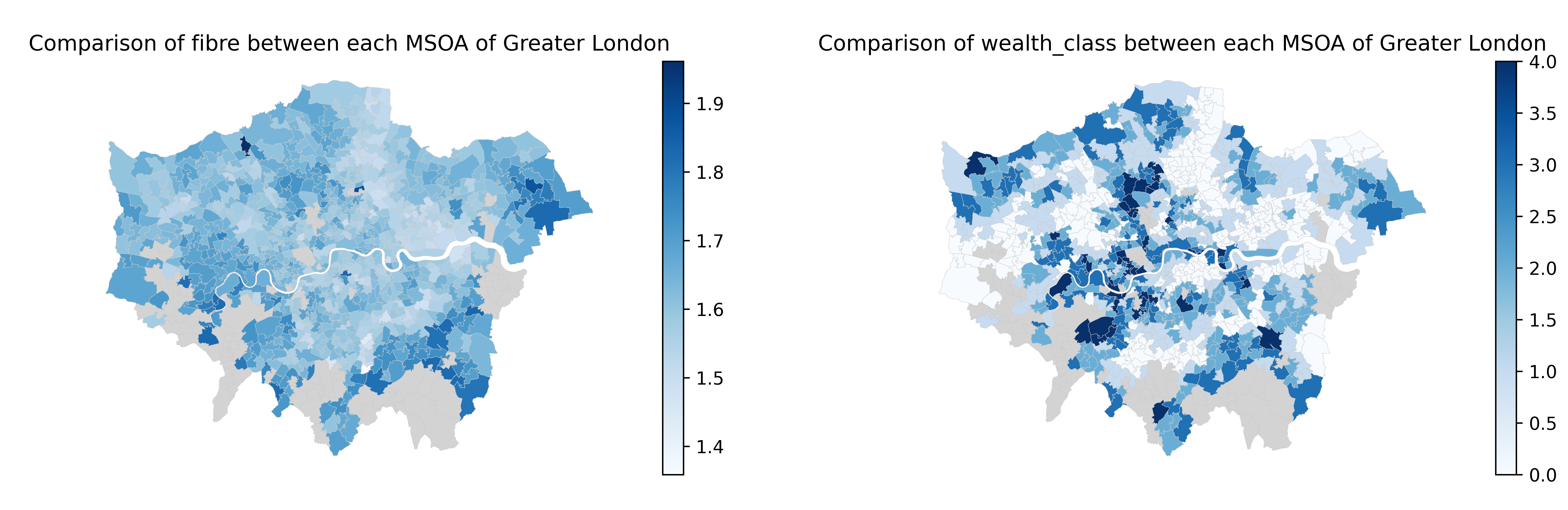
DATA: “As a very last remark, let me underline that the grey areas are the MOSAs that are taken into account due to their low representativeness.”
Mmh ok, it might be good to know. Now let us look at this map.

Interesting… we discern fibre somehow correlates with the wealth class. Especially, remark this lighter diagonal ‘>’ shape (on the right part of the map) that links very low incomes with low weight of fibres in the population’s diet. However, it is quite hard to evaluate how big and significant the correlation is.

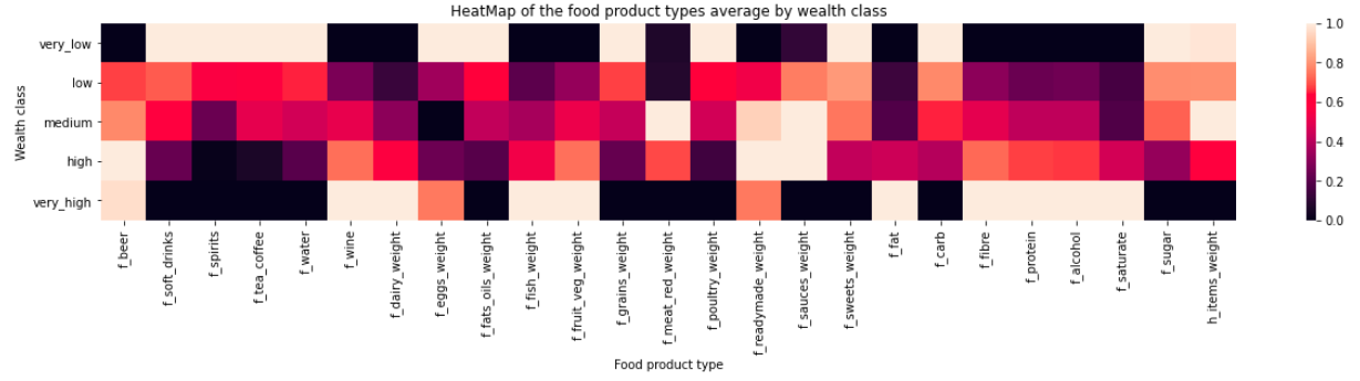
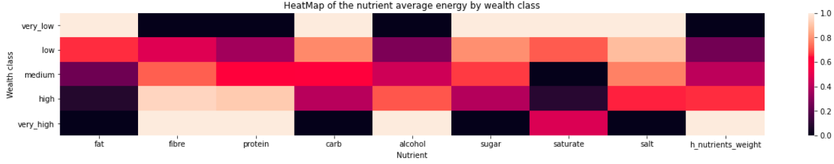
We want to know more! Let’s increase the temperature so DATA shows us beautiful red shades. For each nutrient and product type, we would like to visualize the correlation between their mean weight within each class and the wealth classes.

Amazing DATA!!

DATA: “Hmm, may I say something”?

Well, if it’s interesting, of course!

DATA: “ok, note each f_{product_type}_weight field denotes the fraction of total product weight given by products of type {product_type}”

It’s good to know, next time, be more precise please before plotting! Then what are f_{product_type} and {nutrient} fields?

DATA: “The f_{product_type} fields denote the fractions of product type {product_type} purchased. A {nutrient} field is the weight of {nutrient} in the average product, in grams. So in the heatmap, you see the average value of each of these fields for each wealth class.”

Thank you for these valuable informations. So it seems that the consumption of wine, fish, dairy products, fruit&vegetables and beer are correlated with high social class value, whereas the consumption of soft drinks, spirits, grains, poultry and sweets are correlated with low social class value.

We also observe that fibre, protein, alcohol and the nutrients entropy are correlated with high wealth class whereas salt, fat, carb and sugar are correlated with low class value. Finally, for saturate fat, we don’t observe clear correlation.

It seems that all features which are positively correlated are markers of healthy eating, whereas the features which are negatively correlated are markers of unhealthy eating. But under interrogation, couldn’t DATA tell us a little more about what we want to know?

Let’s make a last visualization before looking for proofs. DATA! Show us the distribution of nutrients for each wealth class!

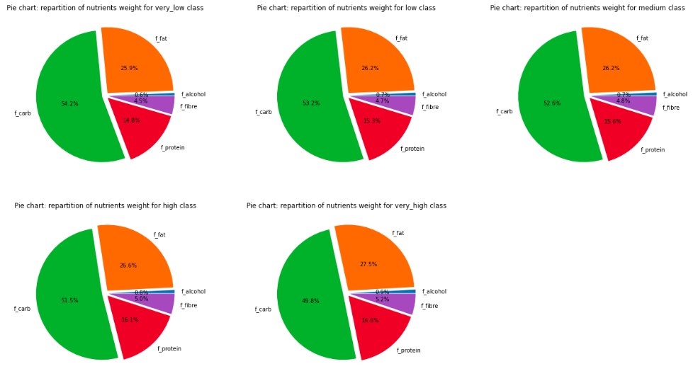
Well, well, well, the differences in proportions are quite small. But if we observe carefully, we see the percentage of protein increases by 0.3% up to 0.6% for each class increase. The same phenomena can be observed for fat, alcohol and fibre, thus the fraction of carb decreases with higher class level. So it seems there are indeed correlations. The differences in eating habits are not huge, however as data analysts, we especially aim to spot those non-obvious facts.

DATA, it’s lies detector time

The correlation test

DATA, we will ask you questions about two sets of features. First, the weigh distribution of purchased product types. Then the mean weight of each nutrient within these products. It’s time to pass the spearman correlation test, we will now if you lie using the p_value. If it is below 0.05, then we will reject your sayings.

Let’s go with product type first:

Well, the above correlations are all statistically significant. DATA is not lying to us, fine!

We note strong positive correlations between wealth class and both fruit&vegetables, dairy and fish which are markers of healthy eating habits. We note strong negative correlation between wealth class and sweets, soft drinks which are marker of unhealthy eating habits.

We also note a strong positive correlation for wine and negative correlation for water (remember this is the volume of bought water so it does not include tap water). Concerning wine, is it not surprising that, as it is wealthy product, its consumption is correlated with the median income. The most likely hypothesis for this second correlation is that the amount of water bought does not vary this significantly but from the fact that wealthier populations buy more products, then the fraction of water seems reduced. Also we need to remember this only concerns the volume of bought water (tap water cannot be taken into account) so making conclusions on it is not an easy task.

Ok DATA, we will now make the same test on nutrients:

Again, all correlations are statistically significant. We indeed note strong positive correlation between both fibre, entropy, protein, and alcohol with median income whereas we note negative correlation with saturate, fat, carb, sugar and salt. If we consider protein, fibre and entropy as health markers, we indeed have a strong correlation health - wealth. Very good job DATA!

The logistic test

Finally, we have a last question. What features would you use to predict the wealth class? Note that by answering this question we will better know whether or not the wealth impacts eating habits, so be clear and concise.

The test will be simple, we will group medium, low and very low class into non wealthy class and group high and very high into wealthy class. By cumulating fraction values of healthy products (dairy, fish, fruit&veg) into healthy and cumulating fraction values of unhealthy products (fats oils, sweets) into unhealthy, could you predict the wealth class DATA ?

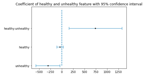
Congratulation DATA, you managed to explain 29% of the variance with those features. Plus the coefficient of unhealthy and the combined unhealthy:healthy are statistically significant having a p_value below 0.05. But we reject healthy as not significant (p_value=0.27). The unhealthy coefficient is negative meaning buying more unhealthy product lowers probability for the MSOA area to be wealthy. Still, note that fraction features are dependent since they sum up to one. That’s why we combined healthy to unhealthy. This last one has positive coefficient and is statistically significant. Combining this to the fact that unhealthy is also significant means that areas where fractions of unhealthy product are going to healthy product have higher probability to be wealthy.

And now the very last test, let DATA launch the same experiment with nutrients and the nutrients weight entropy:

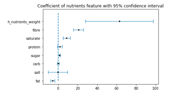
Very good DATA! Now you managed to explain 45% of the variance, we will stick to this version as it is better. All coefficients except salt, protein and carb are statistically significant. Both h_nutrients_weight, fibre, sugar and saturate have positive coefficients whereas fat has negative coefficients. With this, we can conclude entropy and fibre, which are markers of healthy food habits, have the highest influence on the wealth class.

Thank you for your cooperation DATA, we’ll likely see each other again in the next days.

Conclusions and limitations

Let’s recapitulate what we have found so far. We have seen that, at MSOA level in Greater London, there were small in proportion but significant differences in eating habits depending of the wealth level. In particular, we could show that in general wealthier MOSAs buy more fruit, vegetable, dairy and fish while poorer MSOAs correlated with more sweets and soft drinks. Finally, we saw through the last regression (the logistic test) that we could find evidence of social class differences in eating habits (healthier products and nutrients being correlated with wealthier populations).

Now, let’s look at some of the limitations of our work. First of all, we need to remember our study is only conducted on a portion of Greater London population. As London is one of most expensive cities in the world, it is clearly not representative (at all) of the general worldwide population or in the UK. Even if our analysis may yield similar results on other populations, we cannot take this for granted.

A second point to keep in mind is that all the data we used come from Tesco customers (with a fidelity card). Again, this is not representative of the general population as Tesco might better attract some populations or even bias the products they sell (for example Migros does not sell alcohol, similarly Tesco may only have a poor choice of certain food categories).